Jumpstart Your Fabric Environment: A Real Demo on Real Data — in One Line

Jumpstart your Fabric environment with a real demo on real data — in a single line.

import fabric_jumpstart as jumpstart
jumpstart.install("hochschul-insights")

About three minutes later you have a complete German higher-education analytics stack in your workspace — a Lakehouse, a Direct Lake semantic model, an 8-page IBCS report with an Azure Map of all 422 Hochschulen, a pipeline and a Data Agent — all built on real public DESTATIS GENESIS data. No toy sample data, no manual wiring.

This is the first in a new Fabric Demo Series — small, opinionated, end-to-end demos that you can install into your own Microsoft Fabric workspace in a single click and play with right away. More demos coming soon (Defense, Retail, Health, Automotive — all GENESIS-powered).

What is Hochschul-Insights?

A complete German higher-education analytics demo, built on real public DESTATIS GENESIS data, enriched with Wikidata (city + geo) and wrapped in an IBCS-styled Direct Lake report. Eight pages, an Azure Map, a Data Agent for natural-language Q&A, and a single notebook to deploy the whole thing.

Hochschul-Insights report home page

What you get in your workspace

  • Lakehouse hochschul_insights_lh (schemas enabled, schema Genesis) with 16 Delta tables (10 facts, 6 dimensions).
  • Notebooks — an 00_start_here entry point, a snapshot loader, the GENESIS Loader (DESTATIS REST API) and a Wikidata-enriched Dimensions notebook.
  • Data Pipeline hochschul_insights_pipeline orchestrating parallel loads.
  • Direct Lake Semantic Model HochschulInsights with calculated calendar + IBCS measures.
  • Report HochschulInsights — 8 pages, IBCS layout, Azure Map of all 422 Hochschulen.
  • Data Agent hochschul_stats_agent for natural-language Q&A on the model.

Two install modes

The installer supports two flavours, and you pick by whether you paste a token or leave it empty:

  • Snapshot mode (default, no token) — loads bundled CSV snapshots from the public GitHub repo. Fastest path to “look at the report”, no signup needed. Finishes in a few minutes.
  • Live mode (free DESTATIS token) — runs the real pipeline: pulls fresh data from DESTATIS GENESIS, enriches with Wikidata, lands Delta, refreshes the model. ~10–15 minutes end-to-end. Schedule weekly afterwards.

How to install

Hochschul-Insights is now an official community Fabric Jumpstart, so the recommended path is a single line of Python.

Recommended — one line via Fabric Jumpstart

In any Fabric notebook:

%pip install -q fabric-jumpstart

import fabric_jumpstart as jumpstart
jumpstart.install("hochschul-insights")

About 3 minutes later (snapshot mode) the whole stack lands in a single hochschul-insights workspace folder. Then:

  1. Open the hochschul-insights folder and the 00_start_here notebook.
  2. (Optional, live mode only) register at www-genesis.destatis.de, copy your free username token and paste it into the parameters cell. Leave it empty for snapshot mode.
  3. Hit Run all, then open the HochschulInsights report.

No az login, no pip install, no environment variables — the Jumpstart authenticates via notebookutils, auto-detects your workspace and deploys everything. To clean up, just delete the hochschul-insights folder; every item lives inside it.

In live mode you can watch the pipeline run from the same notebook — three parallel GENESIS loads, then the dimensions builder, then the semantic model refresh:

Hochschul-Insights data pipeline

A peek at the report

Eight pages, all IBCS-styled. Here is the live report — click around, it is the real thing (Publish to web, all public DESTATIS data):

Three pages are worth pointing out as you click through the embed above:

  • Home — the landing page: KPIs and a Top-10 university ranking. The hero block here is drawn by a self-made HTML viewer visual (more on that below).
  • Übersicht — totals across all 16 Bundesländer plus an Azure Map of all 422 institutions (lat/lon from Wikidata, City fallback).
  • Studenten — student counts broken down by Fächergruppe, Bundesland, Hochschulart and gender, with cross-filter scenarios baked in.

A self-made IBCS custom visual — built in a few prompts

The multi-tier bar chart on the Studenten page isn’t off-the-shelf — I built that custom visual myself, and that is almost the best part of the story: it went from “I wish Power BI had this” to working-on-the-page in well under an hour, with just a handful of prompts to an AI coding assistant.

It’s a purpose-built IBCS custom visual: AC bars with PY/PL reference markers and Δ / Δ% variance tiers, semantic green/red, all following the IBCS notation standard. It ships in two orientations — horizontal (bar) and vertical (column) — exactly the integrated variance chart the IBCS world loves and stock Power BI doesn’t include. One caveat: at the time of writing it isn’t scrollable yet, so very long category lists get clipped — that’s on the roadmap.

The takeaway: rolling your own Power BI custom visual used to be a side project. With an AI coding assistant it’s an afternoon — often less.

HTML viewer on the Home page

The hero block on the Home page is rendered by an HTML content viewer custom visual: it takes a measure that returns HTML/CSS and renders it live inside the report. That’s how the landing page gets its own typography, KPI tiles and layout without ever leaving Power BI. This one I didn’t build myself — it’s an existing custom visual — but it pairs perfectly with the self-made IBCS chart.

Behind the scenes — what makes this fun

  • Direct Lake on schemas-enabled lakehouse — no import, no scheduled refresh of the model.
  • Wikidata SPARQL for Hochschule geolocation (EF1 + lat/lon, City fallback for the half-dozen missing ones).
  • IBCS measures — units calc group, semantic colours, scenario shading.
  • Loader notebook is pure PySpark + requests + pandas — no add-ons, runs on the default Fabric runtime:
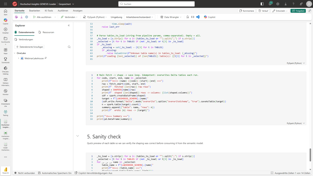
Hochschul-Insights GENESIS Loader notebook

Take it further — build your own

Don’t stop at this demo. Open GENESIS-Online, pick any of the thousands of other tables, swap them into the loader notebook and you have your own end-to-end report in an afternoon. GENESIS is a gold mine: population, labour market, energy, prices, foreign trade, construction, healthcare, agriculture, tax, transport — there is something relevant for every company. Use this demo as the template, point it at the stats that matter for your business, and ship.

Your turn — contribute your solution

The Fabric Jumpstart catalog is a community effort, and this demo is my contribution. Big thanks to Miles Cole for the guidance that got Hochschul-Insights into the catalog — the whole process was smooth because of it. If you have built something end-to-end on Fabric, package it as a Jumpstart so anyone can install it in a single line. So: when will you contribute your solution?

Get it

Fabric Jumpstart (one-line install): jumpstart.fabric.microsoft.com/catalog/hochschul-insights

Source repo: github.com/KornAlexander/hochschul-insights

Data licence (DESTATIS GENESIS): Datenlizenz Deutschland 2.0 — commercial use OK with attribution.

Unlimited Power BI Usage History — Snapshot the Built-In Usage Metrics Model to Lakehouse

Power BI’s built-in usage metrics report is great — until you need history beyond 30 days. The underlying dataset is a rolling window: yesterday’s view counts are there, last quarter’s are gone. If you want to track adoption trends, prove ROI, or spot reports that have quietly died, you need to capture that data yourself.

The fix is surprisingly simple: a single Fabric notebook that queries the hidden Report Usage Metrics Model semantic model over XMLA and appends each daily snapshot to Lakehouse Delta tables. Unlimited history, append-only, ~30 lines of Python.

Usage Metrics Snapshot architecture

Honest Disclaimer — Prefer FUAM

Before you build this: if you have any meaningful scale of Power BI / Fabric tenant, use FUAM (Fabric Unified Admin Monitoring) instead. FUAM is the Microsoft-published, open-source accelerator that snapshots not just usage metrics but capacity events, activity logs, refresh history, inventories — the whole tenant story — into a Lakehouse with a ready-made semantic model and report. It is far more complete than what’s in this post.

So when do I reach for the little notebook below instead?

  • A single workspace where you just need report-level view history and don’t want to deploy a full monitoring solution.
  • You need a quick fix today and FUAM rollout is weeks away.
  • You want to understand how the underlying mechanism works — the notebook is small enough to read end-to-end in five minutes.

For everything else: start with FUAM.

The Problem: 30 Days Is Not Enough

  • Rolling window. Each day, the oldest day falls off. Anything older than 30 days is permanently gone — you cannot recover it.
  • No YoY, no trends. Did adoption grow over the last year? Which reports are losing users? You literally cannot answer these questions with the built-in model.
  • No ownership. Microsoft controls the model. Schema changes happen without notice. You cannot extend it, share it, or join it to your own dimensions cleanly.

The Solution: Daily Snapshot to Lakehouse

The hidden Report Usage Metrics Model is a normal semantic model — it just happens to be auto-managed by Microsoft. That means you can hit it with XMLA queries like any other model. Using sempy.fabric.evaluate_dax, we pull each source table, stamp a SnapshotUtc column, and append to Delta tables in a Lakehouse:

import sempy.fabric as fabric
from datetime import datetime, timezone

WORKSPACE_ID = "<your-workspace-guid>"
DATASET_NAME = "Report Usage Metrics Model"
TABLES = ["Views", "Reports", "Users", "Dates", "DistributionMethods", "Platforms"]

snap_ts = datetime.now(timezone.utc)

for t in TABLES:
    df = fabric.evaluate_dax(
        dataset=DATASET_NAME,
        workspace=WORKSPACE_ID,
        dax_string=f"EVALUATE '{t}'",
    )
    df.columns = [c.split("[")[-1].rstrip("]") if "[" in c else c for c in df.columns]
    df["SnapshotUtc"] = snap_ts.isoformat()
    (spark.createDataFrame(df).write
        .mode("append")
        .option("mergeSchema", "true")
        .saveAsTable(f"usage_metrics_{t.lower()}"))

That’s the whole engine. Schedule it daily after 04:00 UTC (the source refreshes around 03:00 UTC) and you have a permanent historical record.

What Lands in the Lakehouse

One Delta table per source table, prefixed usage_metrics_*, with an extra SnapshotUtc column. Append-only — every run adds today’s full snapshot.

Source tableLakehouse tableRole
Viewsusage_metrics_viewsFact
Reportsusage_metrics_reportsDimension
Usersusage_metrics_usersDimension
Datesusage_metrics_datesDimension
DistributionMethodsusage_metrics_distributionmethodsDimension
Platformsusage_metrics_platformsDimension

Three Design Decisions Worth Calling Out

  • Append, not merge. Every snapshot is the full 30-day window. Yes, days overlap across snapshots — but storage is cheap and append is bulletproof. Deduplication happens at query time (see below), not at ingest time.
  • mergeSchema=true. Microsoft occasionally adds columns to the usage metrics model. With schema merging on, the next snapshot just absorbs the new columns instead of crashing.
  • Retention with DELETE. Default 400 days (≈13 months, enough for YoY) — but you can set RETENTION_DAYS = None to keep forever. The delete is a normal Delta operation, so time travel still works if you mess up.

Querying Without Double-Counting

Because every snapshot contains the last 30 days, the same activity row appears in up to 30 snapshots. To get clean numbers, take the latest snapshot per natural key:

WITH ranked AS (
    SELECT v.*,
           ROW_NUMBER() OVER (
               PARTITION BY Date, ReportGuid, UserGuid
               ORDER BY SnapshotUtc DESC
           ) AS rn
    FROM usage_metrics_views v
)
SELECT Date,
       ReportGuid,
       COUNT(*)                  AS views,
       COUNT(DISTINCT UserGuid)  AS distinct_users
FROM ranked
WHERE rn = 1
GROUP BY Date, ReportGuid
ORDER BY Date DESC, views DESC

For older history (where a date appears in only one snapshot), the deduplication is a no-op — the row simply passes through. For the most recent 30 days, you always pick the freshest version of each fact.

Prerequisites

  • Workspace on Premium / PPU / Fabric capacity (XMLA endpoint enabled — read is enough).
  • The Report Usage Metrics Model dataset exists in the workspace. It is auto-created the first time anyone clicks More options → View usage metrics report on any report in that workspace.
  • A Lakehouse attached to the notebook (any Lakehouse in the same workspace works).
  • Tenant setting “Usage metrics for content creators” enabled (admin portal).

Try It — Fabric Notebook Gallery

The notebook is also submitted to the Fabric Notebook Gallery. Grab the .ipynb directly from GitHub and import it into any Fabric workspace:

📓 Usage Metrics Snapshot.ipynb — one notebook, six Delta tables, daily schedule. Set WORKSPACE_ID, attach a Lakehouse, schedule after 04:00 UTC. Done.

Take It Further — A Power BI Report on Top

The Lakehouse tables are already the hard part. From here, building a proper Adoption & Usage Power BI report is a short hop:

  • Point a Direct Lake semantic model at the six usage_metrics_* Delta tables — no import, no refresh schedule, fresh on the next snapshot.
  • Wrap the "latest snapshot per natural key" dedup logic in a SQL view in the Lakehouse SQL endpoint so the model stays simple. One view per fact, deduped, ready to consume.
  • Build the obvious pages: Adoption over time (views & distinct users by month, YoY), Top & bottom reports, Dying reports (had >X views last year, <Y this quarter), Platform & distribution mix.
  • Join to your own Reports dim (owner, business domain, criticality) for actionable cuts — e.g. "critical reports with zero views in 30 days".

That’s the whole point of owning the history: once the data lives in your Lakehouse, you can model and visualise it however your stakeholders need — not however Microsoft’s built-in report happens to ship it.

Wrap-Up

One notebook, one daily schedule, six Delta tables — and the 30-day blind spot is gone. You own the history, you can join it to your own data, and you can build proper adoption dashboards on top.

The full notebook (with retention, health-check, and example query cells) is on GitHub: KornAlexander/PBI-Tools → Notebook Gallery / Usage Metrics Snapshot.ipynb.